Refit an sdmTMB index under alternative data filters

Refits a fitted sdmTMB::sdmTMB() model once per scenario, each scenario being a rule that drops or modifies data rows (e.g. drop tows shorter than a limit, cap densities at a quantile, drop a cruise series) or a different prediction grid (e.g. restrict the index to an area sampled every year). All refits reuse the model's mesh and every setting of its original call, so only the data or the grid change, and the full model's estimates are used as starting values.

The function is meant for deciding how to handle an anomalous index value: test general rules first, and compare them with a named exclusion of the cruise or survey behind the anomaly. A general rule that removes the anomaly without distorting other years is preferable; an exclusion is defensible when no general rule does, and the scenario table documents why. Haul-level rules (trimming or capping densities, minimum tow length) cannot remove an anomaly that builds up over many moderate hauls of one cruise; use sdmTMB_leave_out() to see whether an anomaly is driven by single hauls or by whole cruises.

Usage

sdmTMB_data_scenarios(
  object,
  scenarios,
  newdata,
  area = 1,
  baseline = "Baseline",
  index = c("plugin", "split"),
  nsplit = NULL,
  bias_correct = FALSE,
  level = 0.95,
  warm_start = TRUE,
  n_workers = 1,
  future_seed = TRUE,
  verbose = TRUE
)

Arguments

object

A fitted sdmTMB::sdmTMB() model.

scenarios

A named list of scenarios. Each element is either

a function of the model data returning a logical vector, TRUE for the rows to keep (e.g. function(d) d$tow_length >= 0.75);
a function returning a data frame with the same rows as the model data and modified values (e.g. densities capped at a quantile); or
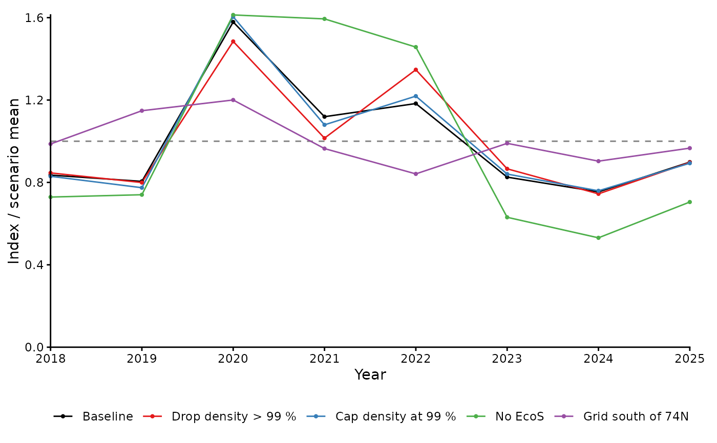
a list with optional elements data (one of the two functions above) and newdata (a prediction grid used for that scenario instead of newdata; its index is not on the same domain as the others, so compare it with plot(x, type = "scaled") or peak_ratio()).

A model fitted with a numeric offset vector keeps the original offset of each kept row, so a scenario that changes effort (e.g. swept area) only changes the offset when the model's offset was given as a column name.

newdata

Prediction grid with the predictors of the fitted model and its time column.

area

Grid cell area: a single value, a column name in the grids, or a numeric vector with one value per row of newdata (only for scenarios that use newdata).

baseline

Character. Name of the reference scenario: a refit to all data on newdata. Default "Baseline".

index

Character. "plugin" (default) or "split" (see sdmTMB_leave_out()).

nsplit, bias_correct, level

Passed to sdmTMB::get_index_split() when index = "split".

warm_start

Logical. Use the full model's estimates as starting values? Default TRUE.

n_workers

Integer. Number of parallel workers. Default 1, which uses whatever future::plan() is currently set. Values > 1 set a temporary parallel plan (forked future::multicore where supported, otherwise future::multisession).

future_seed

Logical or integer. Future-compatible random seed.

verbose

Logical. Show progress messages? Default TRUE.

Value

An object of class sdmTMB_data_scenarios, a list with

index: the index of each scenario by year, with columns scenario, year, est (and lwr, upr, se for index = "split"), ratio (est divided by the baseline) and removed (TRUE for years without data in the scenario, where est is NA);
summary: one row per scenario with n_rows (rows kept), n_modified (rows whose values changed), grid ("own" when the scenario has its own grid), mean_abs_change (mean absolute relative change from the baseline over the years) and all_ok (whether the refit passed sdmTMB::sanity()).

Author

Mikko Vihtakari

Examples

# \donttest{
data(sebastes)
sub <- subset(sebastes, cruiseseries %in% c("EcoS", "WinterS") & year >= 2018)
mesh <- sdmTMB::make_mesh(sub, c("X", "Y"), cutoff = 60)
fit <- sdmTMB::sdmTMB(
  biomass ~ 1, data = sub, time = "year", mesh = mesh,
  family = sdmTMB::tweedie(), spatiotemporal = "ar1",
  offset = log(sub$swept_area)
)
region <- make_survey_prediction_region(sub, crs = 32633)
grid <- sdmTMB::replicate_df(
  make_prediction_grid(region, resolution = 30), "year", unique(sub$year)
)
cap <- function(d) {
  lim <- stats::quantile(d$density, 0.99)
  d$biomass <- pmin(d$biomass, lim * d$swept_area)
  d
}
sc <- sdmTMB_data_scenarios(
  fit,
  scenarios = list(
    "Drop density > 99 %" = function(d) d$density <= stats::quantile(d$density, 0.99),
    "Cap density at 99 %" = cap,
    "No EcoS" = function(d) d$cruiseseries != "EcoS",
    "Grid south of 74N" = list(newdata = grid[grid$Y < 8200, ])
  ),
  newdata = grid, area = (30 / 1.852)^2
)
#> ⠙ Refitting the baseline
#> ✔ Refitting the baseline [6ms]
#> 
#> ⠙ Refitting 4 scenarios
#> ✔ Refitting 4 scenarios [4ms]
#> 
sc$summary
#> # A tibble: 5 × 6
#>   scenario            n_rows n_modified grid  mean_abs_change all_ok
#>   <fct>                <int>      <int> <chr>           <dbl> <lgl> 
#> 1 Baseline              4056          0 main           0      TRUE  
#> 2 Drop density > 99 %   4015          0 main           0.102  TRUE  
#> 3 Cap density at 99 %   4056         41 main           0.0197 TRUE  
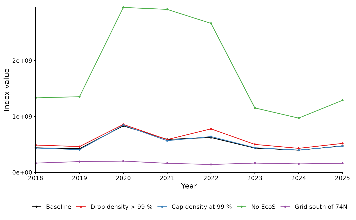
#> 4 No EcoS               2677          0 main           2.35   TRUE  
#> 5 Grid south of 74N     4056          0 own            0.663  TRUE  
peak_ratio(sc, year = 2020)
#> # A tibble: 5 × 4
#>   scenario                   peak  neighbours peak_ratio
#>   <fct>                     <dbl>       <dbl>      <dbl>
#> 1 Baseline             832494220.  507279459.       1.64
#> 2 Drop density > 99 %  858550320.  524704767.       1.64
#> 3 Cap density at 99 %  843973841.  487634508.       1.73
#> 4 No EcoS             2950677485. 2134902773.       1.38
#> 5 Grid south of 74N    202656735.  178340215.       1.14
plot(sc)

plot(sc, type = "scaled")

# }

Usage

Arguments

Value

See also

Author

Examples