Download and Visualize Landings Data

Mikko Vihtakari (Institute of Marine Research)

15 September, 2025

Packages required to run the examples:

# Package names
packages <- c("RstoxUtils", "sf", "dplyr", "ggOceanMaps", "ggplot2", "data.table",
              "lubridate", "tidyr")

# Install packages not yet installed
installed_packages <- packages %in% rownames(installed.packages())
if (any(installed_packages == FALSE)) {
  
  if("RstoxUtils" %in% packages[!installed_packages]) {
    remotes::install_github("DeepWaterIMR/RstoxUtils", upgrade = "never")
  }
  
  installed_packages <- packages %in% rownames(installed.packages())
  install.packages(packages[!installed_packages])
}

# Load the packages to the workspace
invisible(lapply(packages, function(x) {
  suppressPackageStartupMessages(library(x, character.only = TRUE))}))

Introduction

Landings from Norwegian commercial fisheries are delivered to registered landing facilities, which include both fish processing plants and receiving stations. All landings must be documented through a sales note (sluttseddel), which records detailed information about the catch, including species composition, quantity, landing location, and fishing area. These sales notes constitute a primary data source for official catch statistics and are extensively used in fisheries management and stock assessments in Norway. Since there is a general landing obligation in Norway, the terms ‘landings’ and ‘catches’ are used interchangeably even though unrecorded disgards might occur. The data are distributed as .zip archives via the Norwegian Directorate of Fisheries (FDir) website, and are also accessible through the IMR API on the intranet. The API enables searching and filtering without downloading the entire dataset. The downloadLandings() function retrieves sales note data from the IMR API for the period from 2005 onward, while older data are available as Excel files on IMR servers and can be accessed using the readSluttseddelXLS() function. The downloadLandings() function require a connection to the IMR intranet, while readSluttseddelXLS() dataDir can be defined to access the data from anywhere (for example your hard disk if you have copied the data from the server).

Download sales note data from 2005 onward

The downloadLandings() can be used to download sales note data utilizing the IMR API containing data from 2005. Specify the species name in Norwegian (see FDIRcodes$speciesCodes or Table 1 in the Codes and definitions vignette) and years (if you do not want to download all data). In the example, we’ll download sales note data for beaked redfish (Sebastes mentella).

lnd <- downloadLandings("Snabeluer")

The function returns a summary of the data by default that picks the relevant columns from the sales note list to calculate landings. For reference, the summary is a simple dplyr expression:

sales_notes$Produkt %>%
  dplyr::select(
    "Fangst\u00e5r", "SisteFangstdato", "Redskap_kode", "Hovedomr\u00e5de_kode",
    "Lokasjon_kode", "Fart\u00f8ynasjonalitet_kode", "Rundvekt") %>%
  stats::setNames(c("year", "date", "gear_id", "main_area", "sub_area",
                    "nation", "weight")) %>%
  dplyr::mutate(date = as.Date(date, format = "%d.%m.%Y")) %>%
  dplyr::filter(!is.na(weight) & weight > 0) %>%
  dplyr::mutate(month = lubridate::month(.$date), .before = "date") %>%
  dplyr::mutate_at(
    dplyr::vars(main_area, sub_area, gear_id), as.integer)

This vignette does not delve deeper into the structure of sales notes. Once the download is finished, we take the summary element from the sales note list for further analysis:

salesnote_example_data <- lnd$summary

Sales note data figure inspiration

Below are figures the package author uses in assessment reports. Please, feel free to reuse and modify. Thank the author, if you did so :)

Landings by nation and gear (Figure 1):

pnd <- salesnote_example_data %>% 
  group_by(nation, year) %>% 
  reframe(value = sum(weight)/1e6) %>%
  group_by(nation) %>% 
  reframe(mean = mean(value), sd = sd(value)) %>%
  tidyr::replace_na(list(sd = 0)) %>% 
  arrange(-mean) %>% 
  mutate(nation = factor(nation, levels = nation)) 

pn <- pnd %>% 
  ggplot(aes(x = nation, y = mean, ymin = mean, ymax = mean + sd)) +
  geom_col(color = "black", fill = "grey50") + 
  geom_errorbar(width = 0.2) +
  labs(
    x = "Nation code",
    y = "Reported landings (kt ± SD)"
  ) +
  scale_y_continuous(
    expand = expansion(c(0,0.01)),
    sec.axis = sec_axis(~ . *100 / sum(pnd$mean), name = "Percentage of total average landings")
  ) +
  theme_bw(base_size = 12) +
  theme(axis.title.y.right = element_blank())

pgd <- salesnote_example_data %>% 
  left_join(
    FDIRcodes$gearCodes %>% 
      mutate(gearCategory = sub(" ", "\n", gearCategory)),
    by = join_by(gear_id == idGear)) %>% 
  group_by(gearCategory, year) %>% 
  reframe(value = sum(weight)/1e6) %>%
  group_by(gearCategory) %>% 
  reframe(mean = mean(value), sd = sd(value)) %>%
  tidyr::replace_na(list(sd = 0)) %>% 
  arrange(-mean) %>% 
  mutate(gear = factor(gearCategory, levels = gearCategory)) 

pg <- pgd %>% 
  ggplot(aes(x = gear, y = mean, ymin = mean, ymax = mean + sd)) +
  geom_col(color = "black", fill = "grey50") + 
  geom_errorbar(width = 0.2) +
  labs(
    x = "Gear category",
    y = "Reported landings (kt +/- SD)"
  ) +
  scale_y_continuous(
    expand = expansion(c(0,0.01)),
    sec.axis = sec_axis(~ . *100 / sum(pgd$mean), name = "Percentage of total average landings")
  ) +
  theme_bw(base_size = 12) +
  theme(axis.title.y.left = element_blank())

cowplot::plot_grid(pn, pg, labels = "AUTO")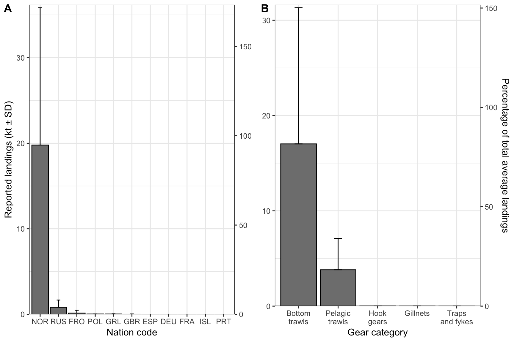

Figure 1: Average annual beaked redfish catches delivered to Norwegian landing facilities by nation (A) and catches by reported gear (B). Error bars indicate standard deviations among years. Catches in kilotons are shown on the left y-axis while the right y-axis indicates the percentage of total average landings.

Geographic distribution of landings (Figure 2). Note how vessels tend to fish outside Norwegian waters and still deliver the fish to Norwegian landing facilities. These landings must be filtered out when doing assessment for a specific region.

tmp <- salesnote_example_data %>% 
  group_by(year, main_area) %>% 
  reframe(value = sum(weight)/1e6) %>% 
  left_join(ggOceanMaps::fdir_main_areas %>% 
              mutate(main_area = as.integer(main_area))) %>% 
  sf::st_as_sf()

p <- ggOceanMaps::basemap(tmp) +
  geom_sf(data = tmp, aes(fill = value)) +
  facet_wrap(~ year, ncol = 3) +
  scale_fill_distiller(
    palette = "Spectral", na.value = "white") +
  labs(fill = "Catch (kt)") +
  theme(legend.position = "bottom",
        axis.title = element_blank(), 
        axis.text = element_blank()
  )

reorder_layers(p)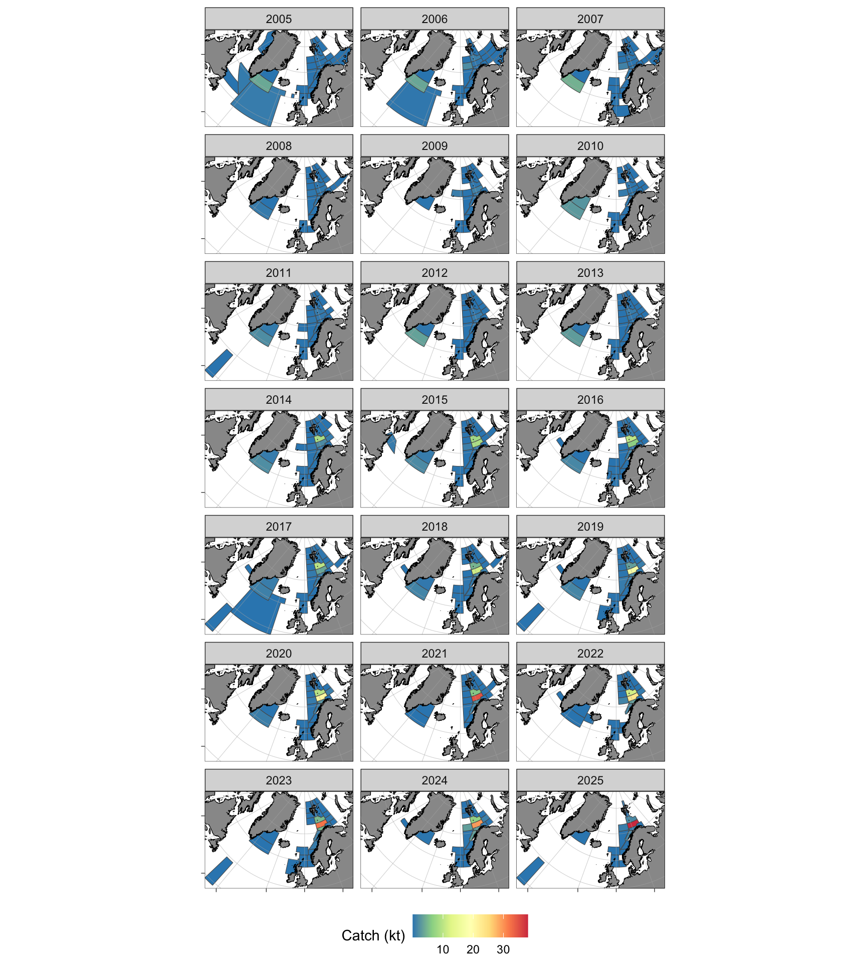

Figure 2: Spatial distribution of beaked redfish landed to Norwegian harbors by year.

The most important figure, annual landings by Norwegian vessels in the assessment area, as international data are accessed through ICES (Figure 3). According to the package author, the main areas (hovedområde) c(0:7, 10:18, 20:27, 30, 34:39, 50) roughly correspond to ICES areas 1 and 2 according to the package author. Please provide feedback, if this correspondence can be improved.

salesnote_example_data %>% 
  filter(
    main_area %in% c(0:7, 10:18, 20:27, 30, 34:39, 50),
    nation == "NOR"
  ) %>% 
  group_by(year) %>% 
  reframe(value = sum(weight)/1e6) %>% 
  ggplot(aes(year, value)) +
  geom_col(color = "black", fill = "grey50") + 
  labs(
    x = "Year",
    y = "Catch (kt)"
  ) +
  scale_y_continuous(expand = expansion(c(0,0.01))) +
  theme_bw(base_size = 12)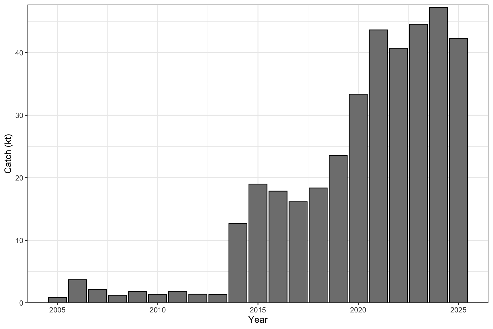

Figure 3: Annual beaked redfish landings by the Norwegian fleet within ICES areas 1 and 2 according to the sales note data.

Sales note data before 2005

Sales note data before 2005, compiled by Hans Stockhausen, are stored as Excel sheets on IMR servers. If you work in Bergen, you can read these files directly from the server with the readSluttseddelXLS() function. In contrast, users in Tromsø may find it easier to copy the relevant folders (“sluttseddel_xls_ferdige_År”) to their own hard disk due to slow server access. Remember, these data are not confidential, unlike ERS data for vessels under 15 meters.

# Path to Stockhausen's sluttseddel Excel files to access data before 2005. 
# If you want to use the server, check his emails for the correct path
sluttseddel_excel_path <- ".../sluttseddel/sluttseddel_XLS_ferdige_År"

salesnote_xls_data <- RstoxUtils::readSluttseddelXLS(
  species = "Snabeluer",
  dataDir = sluttseddel_excel_path)

The lines representing estimated catches overlap demonstrating that the results from these two data sources are almost identical (Figure 4). readSluttseddelXLS() does not include the latest years because the Excel sheets were a mess at time of writing, but it is possible to try opening them by adjusting the years argument.

salesnote_example_data %>% 
  filter(
    main_area %in% c(0:7, 10:18, 20:27, 30, 34:39, 50),
    nation == "NOR"
  ) %>% 
  group_by(year) %>% 
  reframe(value = sum(weight)/1e6) %>% 
  mutate(source = "API") %>% 
  bind_rows(
    salesnote_xls_data %>% 
      filter(
        main_area %in% c(0:7, 10:18, 20:27, 30, 34:39, 50)
      ) %>% 
      group_by(year) %>% 
      reframe(value = sum(weight)/1e6) %>% 
      mutate(source = "Excel")
  ) %>% 
  ggplot(aes(year, value, color = source)) +
  geom_path() +
  labs(
    x = "Year",
    y = "Catch (kt)",
    color = "Source"
  ) +
  scale_y_continuous(expand = expansion(c(0,0.01))) +
  theme_bw(base_size = 12)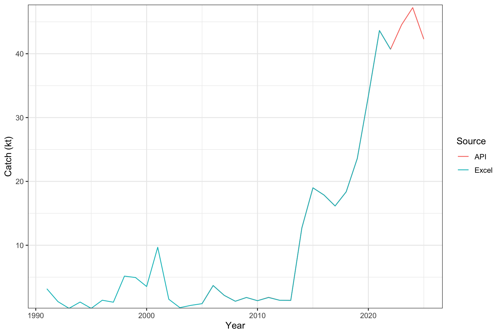

Figure 4: Annual beaked redfish landings by the Norwegian fleet within ICES areas 1 and 2 according to the sales note data acquired using downloadLandings and readSluttseddelXLS.

Troubleshooting

The downloadLandings() function may sometimes return something like:

Error in downloadLandings(“Uer (vanlig)”) : Species code 2202 with years not found from the database.

Even if it worked previously and there is an access to the server. This happens likely (but not confirmed) due to unstable connection to the institute’s intranet (at least in Tromsø). If you are certain that the species exists and you have a connection to the intranet, try running the command again. If it still does not work, try splitting the request to smaller pieces using the years argument.