Download and Visualize ERS Data

Mikko Vihtakari (Institute of Marine Research)

15 September, 2025

Packages required to run the examples:

# Package names
packages <- c("RstoxUtils", "sf", "dplyr", "ggOceanMaps", "ggplot2", "ggspatial",
    "lubridate", "tibble", "tidyr", "hexbin")

# Install packages not yet installed
installed_packages <- packages %in% rownames(installed.packages())
if (any(installed_packages == FALSE)) {
  
  if("RstoxUtils" %in% packages[!installed_packages]) {
    remotes::install_github("DeepWaterIMR/RstoxUtils", upgrade = "never")
  }
  
  installed_packages <- packages %in% rownames(installed.packages())
  install.packages(packages[!installed_packages])
}

# Load the packages to the workspace
invisible(lapply(packages, function(x) {
  suppressPackageStartupMessages(library(x, character.only = TRUE))}))

Introduction

The Directorate of Fisheries in Norway (FDir) collects and distributes data on the exact positions and times of commercial fishing events by the Norwegian fleet for vessels >15 m. These data, referred to as ERS (Electronic Registration System), are available on the FDir website. Currently, the data are only available in Norwegian and are compressed into large, non-searchable zip files. The downloadERS() and extractERS() functions facilitate efficient handling of these datasets.

Download ERS data

The downloadERS() function can be used to download all .zip files listed on the webpage. Specify the dest argument to a location with sufficient storage capacity:

downloadERS(dest = "~Documents/Fisheries data/FDIR ERS data",
            years = c(2011, 2018, 2025))

In this example, only the years 2011, 2018, and 2025 are used to conserve space. However, you may omit the years argument to download all available data from 2011 onward.

Process ERS data

After downloading, use the extractERS() function to read the data:

ers_example_data <- 
  extractERS(path = "~Documents/Fisheries data/FDIR ERS data",
             species = "snabeluer")

The data can now be visualized and used for further analysis:

pp <- ggOceanMaps::basemap(
  ers_example_data, bathy.style = "contour_grey", base_size = 12) +
  stat_summary_hex(
    data = ers_example_data %>%
      ggOceanMaps:: transform_coord(bind = TRUE),
    aes(x = lon.proj, y = lat.proj, z = weight/1e3), bins = 30,
    fun = "sum") +
  scale_fill_distiller(
    palette = "Spectral", na.value = "grey", limits = c(0, NA),
    trans = "sqrt")  +
  facet_wrap(~year, ncol = 1) + 
  labs(x = NULL, y = NULL, fill = "Catch (t)") + 
  theme(
    legend.box.margin = margin(0, 0, 10, 0),
    legend.background = element_rect(fill = "transparent", color = NA),
    legend.box.background = element_rect(fill = "transparent", color = NA))

reorder_layers(pp)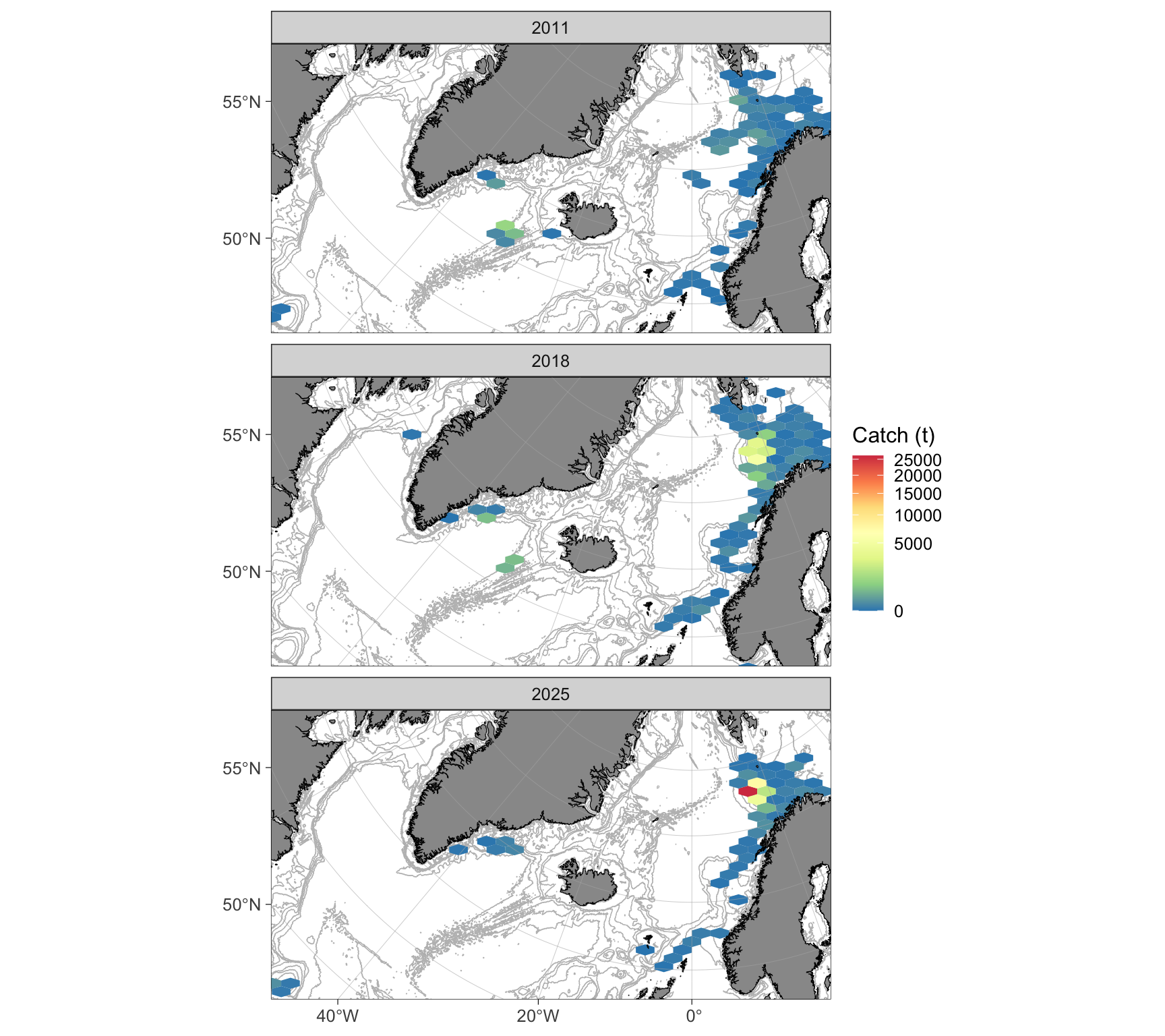

Figure 1: Spatial distribution of total beaked redfish catches by the Norwegian fleet (>15 m) based on ERS data. Facets represent different years. The color scale, indicating aggregated total catches in tons, has been square-root transformed.

ers_example_data %>% 
  mutate(gear = case_when(
    grepl("Bunntr|Udefinert tr|Snurrevad", gear) ~ "Bottom\ntrawls",
    grepl("Reketr", gear) ~ "Shrimp\ntrawls",
    grepl("Flytetr", gear) ~ "Pelagic\ntrawls",
    grepl("Garn", gearGroup) ~ "Gillnets",
    grepl("Krokredskap", gearGroup) ~ "Hooks",
    .default = "Other"
  )) %>% 
  group_by(year, gear) %>% 
  reframe(value = sum(weight)/1e3) %>% 
  group_by(gear) %>% 
  mutate(total = sum(value)) %>% 
  arrange(-total) %>% 
  mutate(gear = factor(gear, levels = unique(.$gear))) %>% 
  ggplot(aes(x = gear, y = value)) +
  geom_col() +
  facet_wrap(~ year) +
  labs(x = "Gear category", y = "Catch (t)") +
  theme_bw(base_size = 12)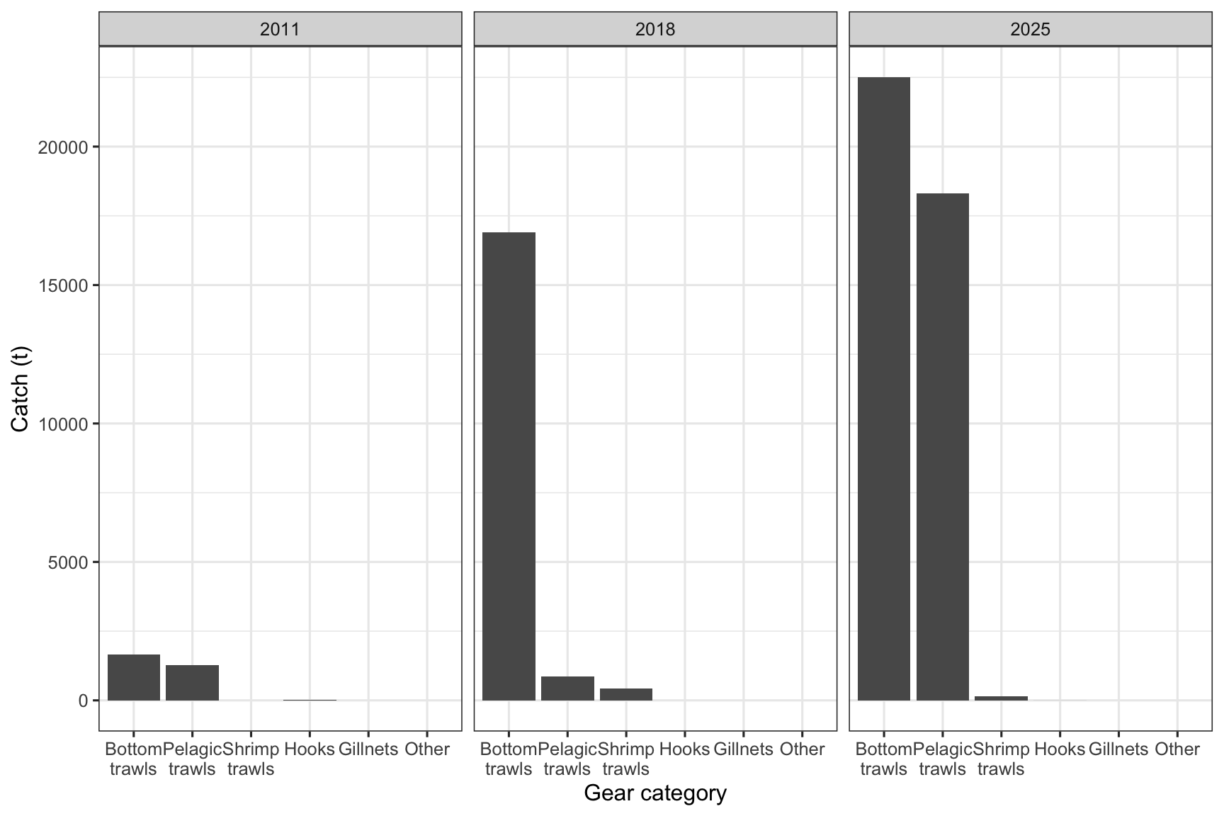

Figure 2: Beaked redfish catches by gear type and year based on ERS data for the Norwegian fleet (>15 m).

x <- ers_example_data %>% 
  filter(grepl("Bunntr|Udefinert tr|Snurrevad|Reketr|Flytetr", gear)) %>% 
  filter(grepl("27_2_|27_1_", ICESArea)) %>% 
  mutate(gear = case_when(
    grepl("Flytetr", gear) ~ "Pelagic trawls",
    .default = "Bottom trawls"
  ))

ggOceanMaps::basemap(x, base_size = 12, bathy.style = "contour_grey") +
  ggspatial::geom_spatial_point(
    data = x %>% 
      mutate(weight = weight/1e3),
    aes(x = lon, y = lat, size = weight),
    color = "red", shape = 21, alpha = 0.5, stroke = LS(1)) +
  scale_size_area(
    max_size = 12,
    breaks = c(1,5,10,20,40,60.80)
    ) +
  labs(x = NULL, y = NULL, size = "Catch (t)") + 
  facet_wrap(~gear) + 
  guides(size = guide_legend(nrow = 1)) +
  theme(legend.position = "bottom",
        legend.box.margin = margin(0, 0, 10, 0),
        legend.background = element_rect(fill = "transparent", color = NA),
        legend.box.background = element_rect(fill = "transparent", color = NA))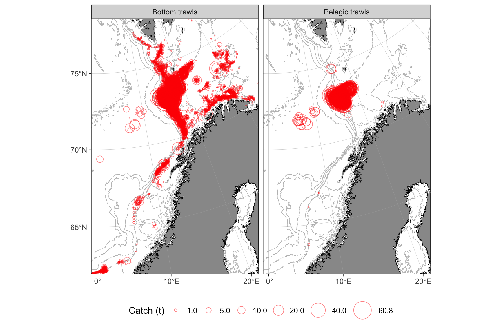

Figure 3: Spatial distribution of beaked redfish catches by bottom and pelagic trawls within the Northeast Arctic (ICES areas 1 and 2) stock, based on ERS data for the Norwegian fleet (>15 m). Data are aggregated across 2011, 2018, and 2025

Accessing data for vessels <15 m

ERS data for vessels <15 m (elFangstdagbok_detaljert) are also available on IMR servers. These datasets are distributed in .psv format. You can use the extractLogbook function to access them. Please note that this function has not been updated since 2021 and may require further development.

These data are confidential and require a special access to the folder on the server where they are located. If you need such access (and work at IMR), take contact with the data people at your group. Those who have the access, know where the data are located. The path argument should point to the folder of interest on the server (elFangstdagbok_detaljert for all data). The path can be defined on Mac (and Linux) as path = "/Volumes/.../elFangstdagbok_detaljert" and as path = Q:/.../elFangstdagbok_detaljert on Windows, where ... represents the entire folder path that cannot be shown here. You can copy the folder location as path to your clip-board and past it the extractLogbook() function. Remember to use quotes (i.e. " ").

The function is slow especially in Tromsø (prepare for 30 min to 1 h). It filters species out of the logbook data based on codes listed in the table under. For example, all Atlantic halibut can be extracted as follows:

extractLogbook(path, species = "HAL")

Or as:

extractLogbook(path, species = 2311) # Excluding farmed fish

The species name will be returned in Norwegian, English or Latin depending on the language argument.