Estimation of strata with RstoxStrata
Mikko Vihtakari (Institute of Marine Research)
10 November, 2022
Source:vignettes/RstoxStrata.Rmd
RstoxStrata.RmdPackages required to run the examples:
library(sf)
library(dplyr)
library(tidyr)
library(tibble)
library(RstoxStrata)
library(ggOceanMaps)
library(cowplot)
Introduction
Fisheries assessment models use catch data and population trends to estimate the fishing quota (Total Allowable Catch, TAC), i.e., the safe or optimal biomass to remove from a population to ensure sustainable fishing. While catch data primarily govern the absolute levels in TAC estimates, population trends dictate the relative changes in TAC from year to year and help the assessment model differentiate fishing effort- and efficiency-related catch variations from actual population fluctuations. Therefore, estimating population trends is integral to fisheries assessment and can have considerable economic and ecologic consequences.
Estimating population trends requires deciphering how much fish there is in the sea, commonly done using survey indices tailored for a particular species, region, and sampling setup. In essence, these survey indices are estimated by summing up numbers or weights of fish within areas called strata. The strata model distribution of a stock within a particular region of interest - often delimited by political or population boundaries. Most survey indices use multiple strata, assuming that the abundance of a species, population structure, or sampling setup considerably differs within the region of interest. The formula for estimating the number (or weight) of fish within a stratum for gear that covers an area, such as trawls, multiplies an average number of fish per areal unit (=density) by area of the stratum. In other words, the density of fish in each stratum is weighted by the area. Since the area is a multiplier, it considerably impacts the outcome. Imprecision in the areal estimation of strata or missing samples within a stratum may greatly affect the estimated population trends and hence TAC.
Depth is among the best factors to describe the distribution of fish species [REFS]. Consequently, bottom depth intervals are commonly incorporated into strata to model the vertical distribution of a species. Using bottom depth can lead to imprecision in areal estimation for species that inhabit narrow depth ranges along the continental slopes, such as the Greenland halibut. Imprecision in the areal estimation stemming from poorly charted bathymetry and low or inconsistent model resolution can be an order of magnitude and directly proportional to survey index estimates.
Here we suggest a transparent framework to estimate strata from bathymetric grid data programmed to an R package called RstoxStrata, which is integrated into the StoX software for survey index calculation. We discuss pitfalls in making strata for survey indices, allocating stations to strata and using them to calculate survey indices. We use the main survey for Northeast Arctic Greenland halibut as an example contrasting two approaches to allocate stations to strata: a bottom depth-latitude based approach used in the current assesment model, and a solely position-based approach used by the StoX software. While the framework is applied to bottom depth, it can be used for any gridded spatial data such as surface temperature, salinity, or modeled prey density.
Material and methods
The proposed way of defining strata attempts to simplify the strata making. Further, the process is transparent and reproducible. The distribution of a species is modeled using two components: 1) geographic regions (rectangles, called geostrata) are used to model the spatial distribution, and 2) bottom depth intervals within the geographic regions are used as a proxy of the vertical distribution. The depth data are acquired from the highest openly available evenly gridded depth model at the time of writing, the General Bathymetric Chart of the Oceans 15-arcsecond 2022 grid (approximately 1/4 nautical miles in the latitude direction). The GEBCO_2022 Grid (ice surface elevation) netCDF file is downloaded (4 Gb) and placed in a central location on the computer:
link <- "~/Downloads/gebco_2022/GEBCO_2022.nc"We use the “EggaNord” survey in the Northeast Atlantic spawning grounds of Greenland halibut as an example. The survey and its strata system are used to estimate the primary stock index for Northeast Arctic Greenland halibut. The original system assigns stations to strata based on latitude and bottom depth at the beginning of trawling [@Høines2008], while the StoX software uses position only in the assignment [@Johnsen2019] (Table 1). The calculus for areas of the strata used in the original system has been lost and is not reproducible. Since the new StoX based approach uses solely position in station allocation to strata, we need to define the longitude limits as well to mimic the old strata system.
| 76-80 | 73.5-76 | 70.5-73.5 | 68-70.5 | |
|---|---|---|---|---|
| 1000-1500 | 2693 | 1672 | 3272 | 945 |
| 700-1000 | 1263 | 761 | 1706 | 1150 |
| 500-700 | 702 | 488 | 1324 | 525 |
| 400-500 | 1440 | 575 | 1228 | 400 |
Geostrata
The geographic rectangles, called “geostrata”, are defined as a data frame for the RstoxStrata package. Optionally, the first column of the data frame can define the names of the geostrata. The four following numeric columns are required and define the minimum and maximum longitude as well as minimum and maximum latitude for the rectangles, respectively (Figure 1). The coordinates are defined in decimal degrees (WGS84 / EPSG:4326).
geostrata.df <- data.frame(
  lon.min = c(3, 10, 10, 8),
  lon.max = c(16, 17.5, 17.5, 17.5),
  lat.min = c(76, 73.5, 70.5, 68),
  lat.max = c(80, 76, 73.5, 70.5)
)

plotGeostrata(geostrata.df)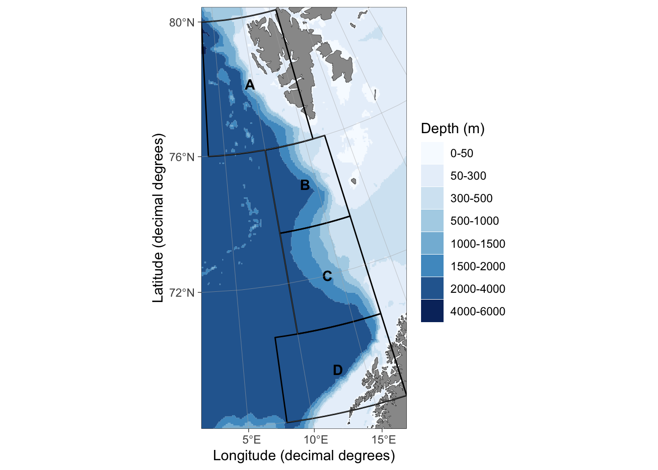
Figure 1: A geostrata system attempting to mimic the EggaNord survey strata for Northeast Greenland halibut. The official system uses latitude and bottom depth at the beginning of trawling for station allocation while the new StoX based approach uses position only.
Depth strata
The depth strata are defined as a numeric vector specifying the cut points for the depth intervals.
depths.vec <- c(400, 500, 700, 1000, 1500)Strata estimation
The GEBCO bathymetry model covers the entire world. Clipping the grid to a region of interest greatly reduces up the computation time. The clipping is done using the boundary argument which accepts vectors with four numbers in the same order than geostrata (minimum and maximum longitude, minimum and maximum latitude).
boundary.vec <- c(0, 17.5, 68, 80)These information can then be input into the strataPolygon() function which performs the strata estimation. The function returns a strataPolygon object, which is a list containing strata and geostrata sf polygon objects. strataPolygon objects have their own plotting method utilizing the ggOceanMaps package, but you can also plot the sf objects using standard syntax.
pols <- strataPolygon(
  bathy = link,
  depths = depths.vec,
  boundary = boundary.vec,
  geostrata = geostrata.df
)

plot(pols)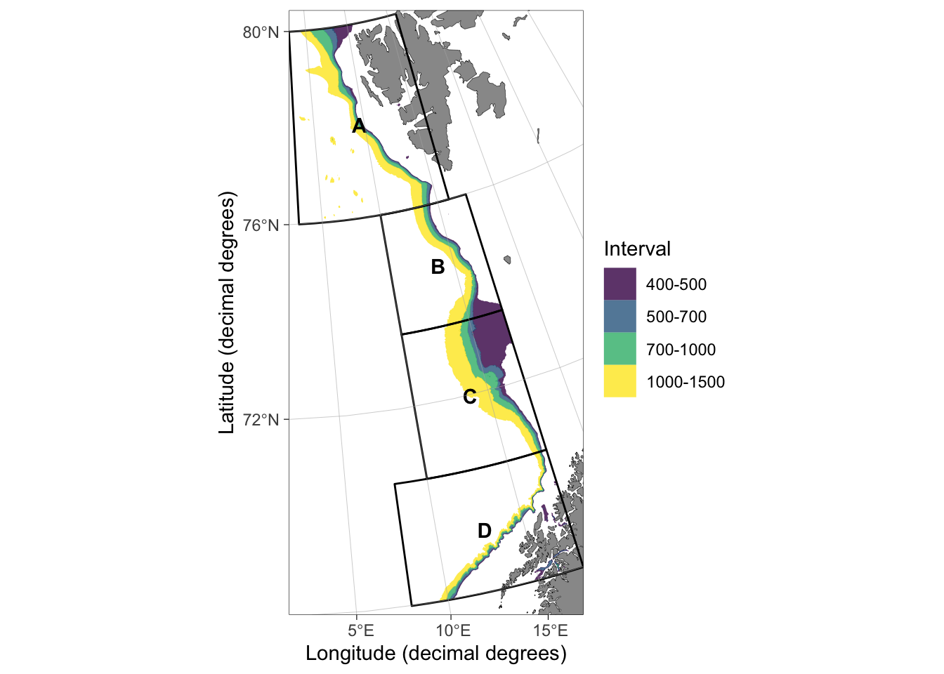
Figure 2: Initial strata system for the EggaNord survey index containing fragments that increase the strata area
The depth strata 400-500 m between geostrata B and C is large and exceeds regularly visited stations. The strataPolygon() function accepts polygons as the boundary argument allowing manual tuning of the strata (Figures 3 and 4). We formulate a spatial polygon using QGIS and tune the polygon such that the estimated area of C 400-500 m matches the official area. The polygon is included in the RstoxStrata package as example data:
boundary <- sf::read_sf(system.file("shapes", "boundary_shape.shp", package = "RstoxStrata"))

ggOceanMaps::qmap(boundary)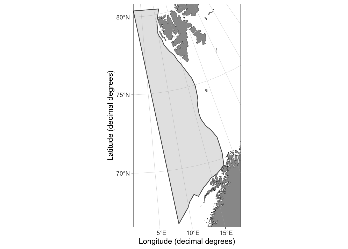
Figure 3: Spatial polygons can be used as the boundary argument within strataPolygons() to manually restrict the strata extend.
The initial strata system contains fragments from sea mounts and fjords. These fragments bias the area of strata and can be removed using the fragment.area argument which accepts a single threshold in square kilometers. Fragments smaller than the threshold will be removed. The process of finding the correct threshold is iterative.
pols <- strataPolygon(
  bathy = link,
  depths = depths.vec,
  boundary = boundary,
  geostrata = geostrata.df,
  fragment.area = 400
)

plot(pols, facetted = TRUE)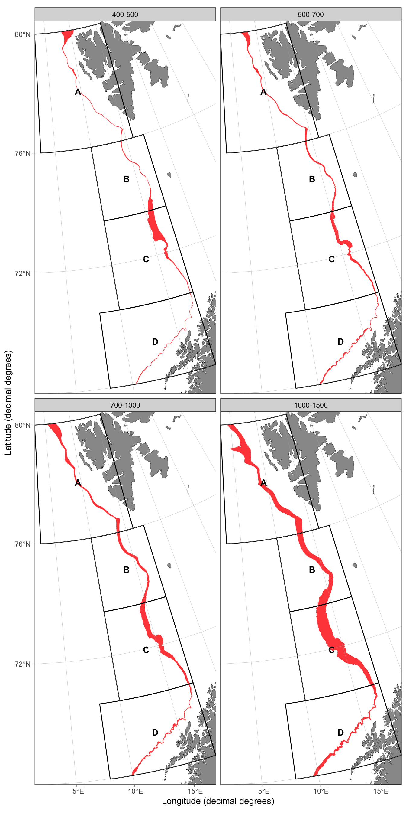
Figure 4: Final strata system for the EggaNord survey to estimate a survey index for Northeast Arctic Greenland halibut. The strata system attemps to mimic the system used in the assessment that bases on latitude and gear depth.
Survey index
Trawl data from the EggaNord survey was used to calculate the survey indices. Biomass of Greenland halibut in all trawl hauls taken during the survey from 1994 until 2021 are included in the data(eggan_ghl) dataset. Swept area density (\(\rho\), called density in the dataset) was calculated as biomass in kg per square nautical mile assuming 80 m as the effective fishing width for all trawls:
\[\rho_i = (\frac{B_i [kg]}{d_i [nmi] * (80 [m]/1852 [m]) [nmi]}) [kg/nmi^2]\] Where i is a trawl station, \(B_i\) biomass of Greenland halibut, and \(d_i\) trawling distance on that stations. Units are given in square brackets.
Indices for each stratum were calculated as average \(\rho\) for a stratum multiplied by area of the stratum.
\[ I_s = (A_s [nmi^2] \times \sum_{i=1}^n \frac{\rho_i [kg/nmi^2]}{n}) [kg]\] Where s is a stratum, \(A_s\) area of that stratum, i a trawl station, and n number of stations within the stratum.
The indices for each stratum were then summed up to formulate an annual survey index value.
\[ I_y = \sum_{s=1}^{n_s} I_s\] Where y is a year, s a stratum, and \(n_s\) number of strata included in the survey index. This survey index is referred to as “recalculated” index to separate it from the official numbers that have directly been acquired from the assessment model. The recalculated index was compared to the official numbers to confirm the calculus.
The survey index calculations have been done using the hidden code under:
Code for survey index calculations
data(eggan_ghl)

stn <- eggan_ghl %>%
  mutate(depth.interval =
           cut(.$bottomdepthstart, depths.vec,
               labels = paste(depths.vec[1:(length(depths.vec)-1)],
                              depths.vec[2:(length(depths.vec))], sep = "-"))
  ) %>%
  st_as_sf(coords = c("longitudestart", "latitudestart"), crs = 4326, remove = FALSE) %>%
  rownames_to_column("id") %>%
  st_join(pols$strata[, c("interval", "geostrata.name", "area.nm2")]) %>%
  filter(!duplicated(id)) %>%
  st_join(pols$geostrata[, c("geostrata.name")] %>%
            rename("geostrata.polygon" = "geostrata.name")) %>%
  filter(!duplicated(id)) %>%
  st_set_geometry(NULL) %>%
  mutate(area.nm2 = as.numeric(area.nm2)) %>%
  left_join(.,
            eggan_ghl_original_strata %>%
              dplyr::select(geostrata.name, interval, orig.nm2) %>%
              rename("geostrata.polygon" = "geostrata.name", "depth.interval" = "interval")
  ) %>%
  rename("area.new" = "area.nm2", "area.old" = "orig.nm2") %>%
  relocate(distance, biomass, density, .after = last_col()) %>%
  suppressMessages()

old_area_old_assig <- stn %>%
  filter(!is.na(area.old)) %>%
  dplyr::select(startyear, geostrata.polygon, depth.interval, area.old, density) %>%
  rename("geostrata.name" = "geostrata.polygon",
         "interval" = "depth.interval",
         "area" = "area.old") %>%
  group_by(startyear, geostrata.name, interval, area) %>%
  summarise(mean = mean(density), sd = sd(density), n = n()) %>%
  mutate(index = area*mean/1e6) %>%
  suppressWarnings() %>%
  ungroup() %>%
  group_by(startyear) %>%
  summarise(reconst = sum(index))

surv_diff <-
  left_join(official, old_area_old_assig %>% rename("year" = "startyear")) %>%
  mutate(diff = value - reconst)

removed_stn <- stn %>% filter(is.na(area.new) | is.na(area.old)) %>%
  mutate(
    reason =
      ifelse(is.na(depth.interval) & is.na(geostrata.polygon), "Both",
             ifelse(is.na(depth.interval), "Depth",
                    ifelse(is.na(geostrata.polygon), "Outside",
                           ifelse(is.na(interval), "Position" ,"Other")))))
pb_index <- stn %>%
  filter(!is.na(area.new)) %>%
  rename("geostrata" = "geostrata.name",
         "area" = "area.new") %>%
  group_by(startyear, geostrata, interval, area) %>%
  summarise(mean = mean(density), sd = sd(density), n = n()) %>%
  mutate(index = area*mean/1e6,
         index.sd = area*sd/1e6,
         ci.min.t = index - qt(1 - 0.025, (n - 1))*index.sd/sqrt(n),
         ci.max.t = index + qt(1 - 0.025, (n - 1))*index.sd/sqrt(n)) %>%
  mutate(type = "Position", .after = "interval") %>%
  mutate(interval = factor(interval, levels = levels(stn$interval))) %>%
  suppressWarnings() %>%
  ungroup()

db_index <- stn %>%
  filter(!is.na(area.new)) %>%
  dplyr::select(-interval) %>%
  rename("geostrata" = "geostrata.polygon",
         "interval" = "depth.interval",
         "area" = "area.new") %>%
  group_by(startyear, geostrata, interval, area) %>%
  summarise(mean = mean(density), sd = sd(density), n = n()) %>%
  mutate(index = area*mean/1e6,
         index.sd = area*sd/1e6,
         ci.min.t = index - qt(1 - 0.025, (n - 1))*index.sd/sqrt(n),
         ci.max.t = index + qt(1 - 0.025, (n - 1))*index.sd/sqrt(n)) %>%
  mutate(type = "Depth-latitude", .after = "interval") %>%
  mutate(interval = factor(interval, levels = levels(stn$interval))) %>%
  suppressWarnings() %>%
  ungroup()
Results
Difference in area
The reconstructed strata areas were lower than the original for approximately half of the strata (Figure 5, Table 2). Area of the deepest 1000-1500 strata, the manually adjusted strata C 400-500, geostrata A excluding the shallowest 400-500 strata, and strata B 700-1000 were within \(\pm\) 7% of the original strata system.
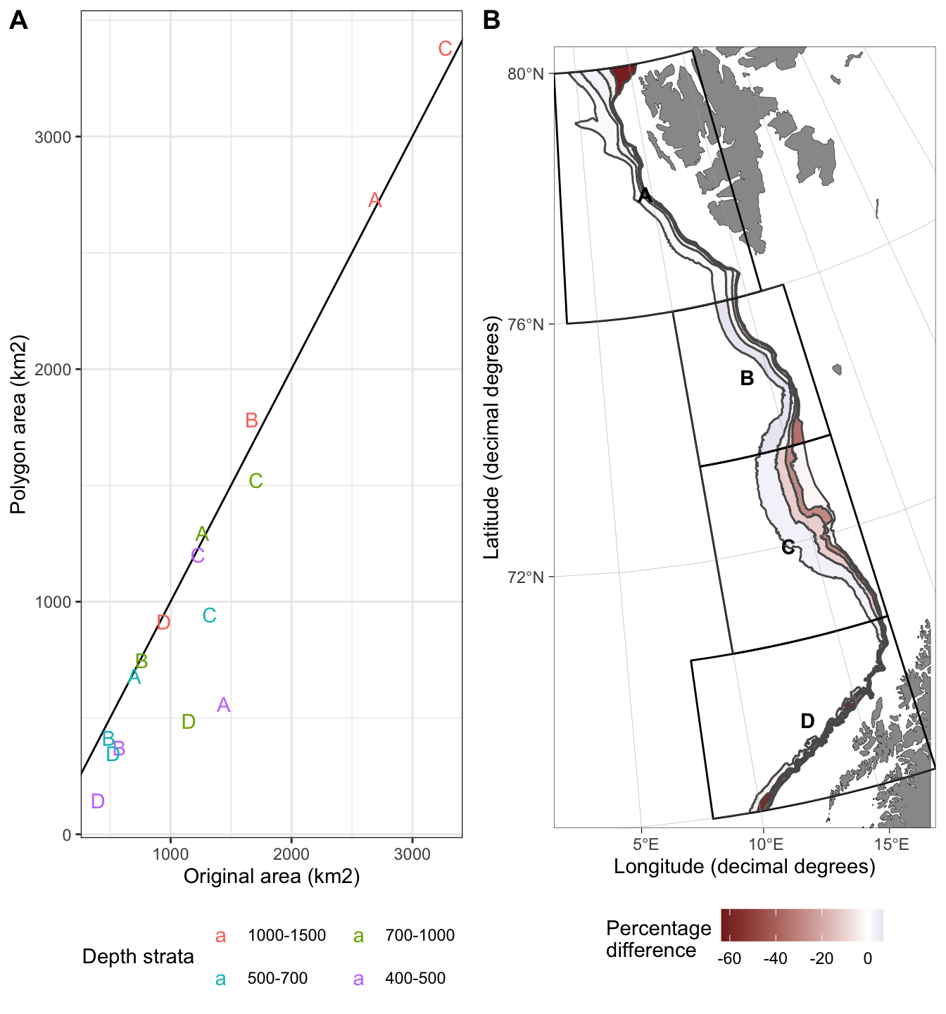
Figure 5: Difference between the original and reconstructed strata area. A) The differences are shown as a scatter plot. Color refers to depth strata and letter to geostrata name. B) The differences are shown on a map. Color refers to percentage difference. Negative percentages mean larger original area than reconstructed area.
| A | B | C | D | |
|---|---|---|---|---|
| 1000-1500 | 1.4 | 6.6 | 3.3 | -3.2 |
| 700-1000 | 2.7 | -2.0 | -10.8 | -57.6 |
| 500-700 | -3.2 | -15.0 | -28.6 | -34.0 |
| 400-500 | -61.2 | -35.1 | -2.1 | -63.6 |
Station assignment difference
Total of 228 stations (6.5%) were assigned differently between depth-latitude- and position-based assignment. Stations were consistently assigned to the same geostrata, but assignment to depth strata differed. Most of these stations had a bottom depth close to the depth strata boundaries (Figure 6), although some had bottom depths that were far off from the depths estimated based on position.
The agreement between depth-latitude and position-based station assignment to strata varied between 84 and 98 (Figure 7). The use of position based station assignment to strata led to removal of 30 stations that were included in the depth-latitude based assignment (Figure 8).
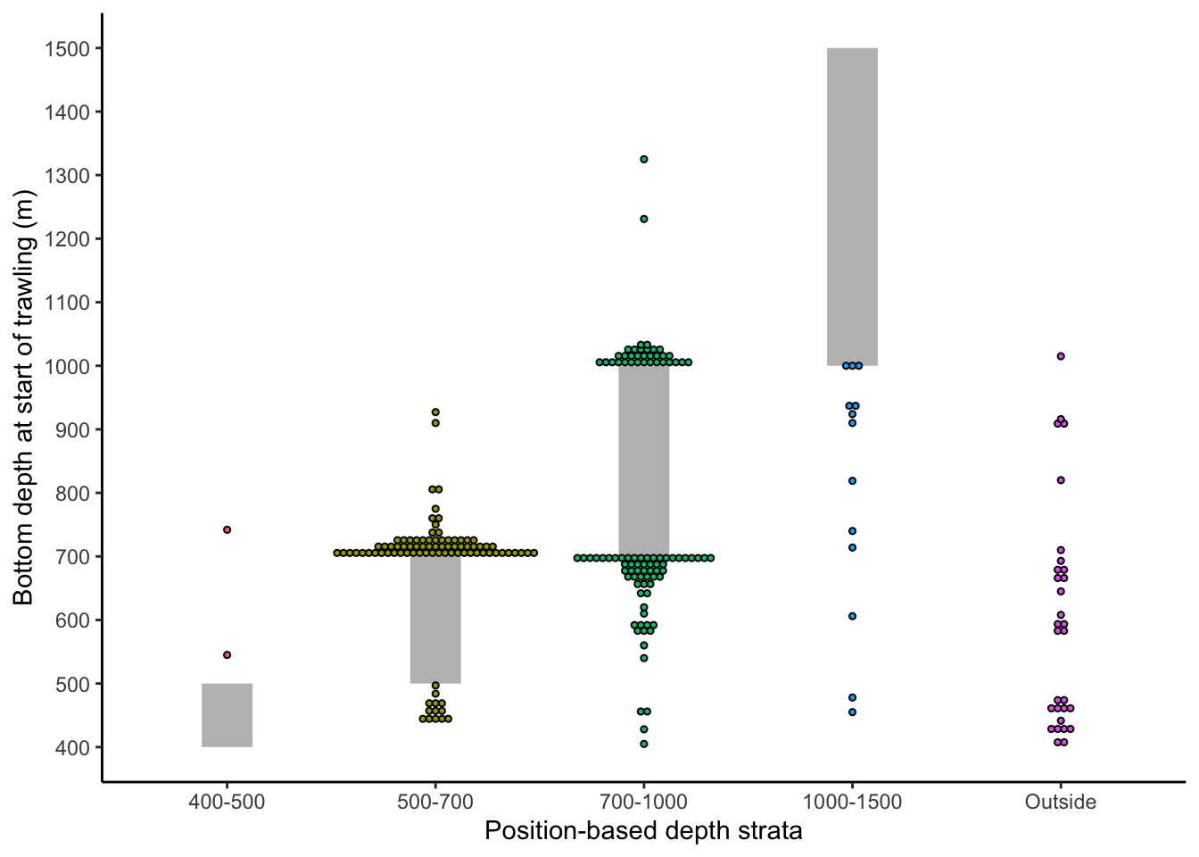
Figure 6: Bottom depth at start of trawling for stations that did not get assigned to the same depth strata between depth-latitude- and position-based assignment. Position-based strata are shown on the x-axis together with the depth interval (grey bar). Dots represent stations. The color of dots indicates position-based strata.
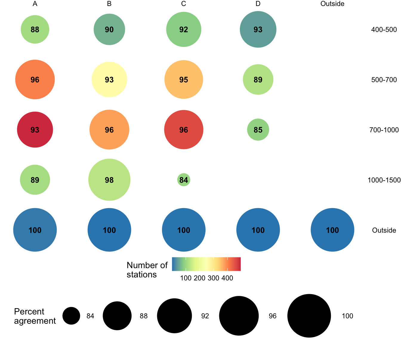
Figure 7: Percent agreement in station allocation to strata between the depth-latitude-based (current assessment) and position-based (StoX) assignment. Size of the bubbles and number inside them refer to the percentage. Fill of the bubbles refer to number of stations. The figure contains all stations sampled during the EggaN survey 1004-2021. Geostrata are shown vertically and depth intervals horizontally.
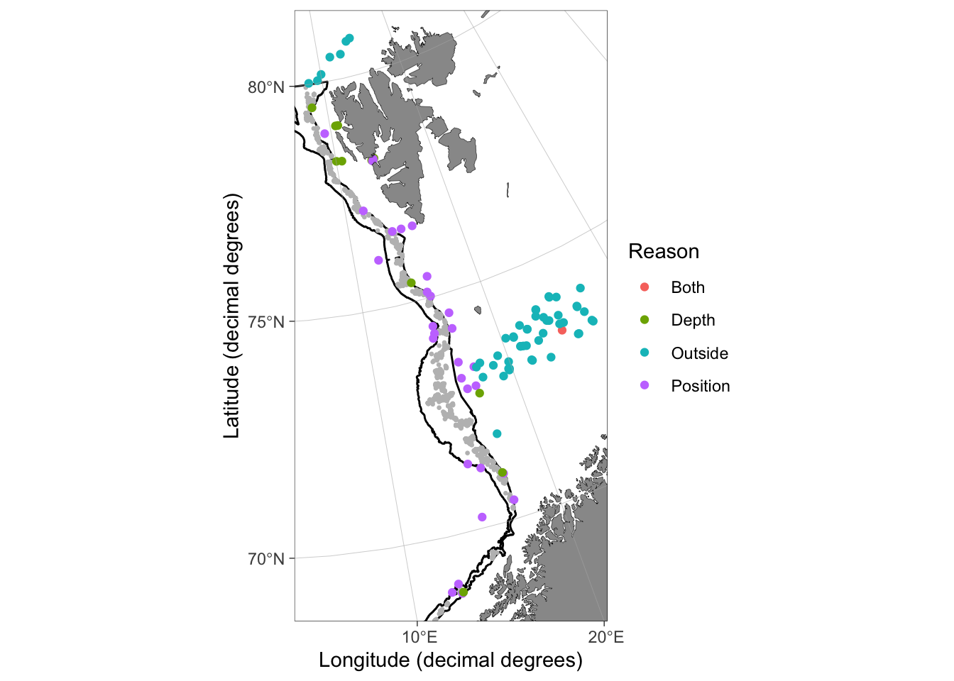
Figure 8: Position of EggaN survey stations removed from survey index calculations. The color indicates the reason for removal: depth = the recorded bottom depth is outside the depth strata; outside = position of the station is outside the geostrata; position = position of the station is outside the strata due to impression in bathymetry model and strata estimation or due to wrongly recorded coordinates; and both = both conditions ‘depth’ and ‘outside’ apply. Grey dots indicate stations included in survey index calculations. The figure contains data from all years (1994-2021).
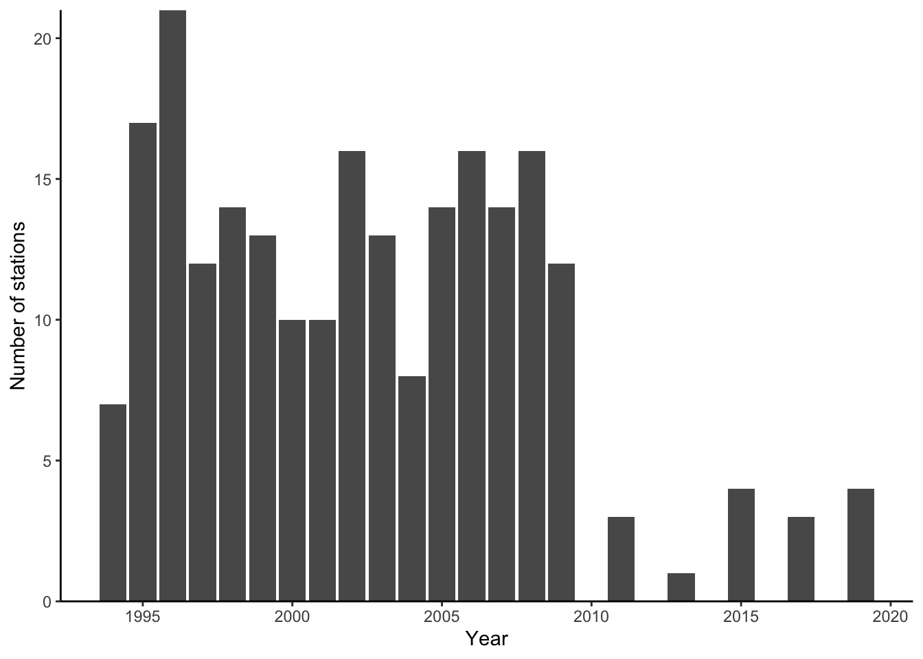
Figure 9: Number of EggaN stations per year that get assigned to different depth strata between the depth-latitude- and position-based regimes.
Difference in survey index
The reconstructed survey index using depth- and latitude-based station assignment to strata and the original strata areas had a Pearson correlation of 0.997 with the official EggaN survey index used in the assessment model (Figure 10A). The average annual difference between these indices was 38 tons and standard deviation 1189 tons (Figure 10B). For comparison purposes the official and reconstructed survey indices were practically identical. The difference is likely caused by a few stations being included/removed from survey index calculations differently and highlights the differences weighing by the area can cause to survey indices. Only the reconstructed survey index is used in the comparison for consistency.
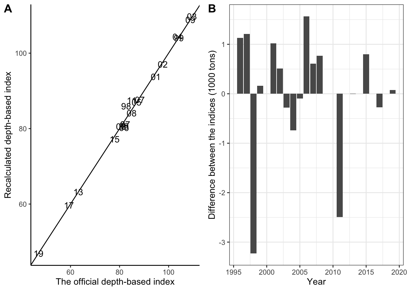
Figure 10: Comparison between the official EggaN survey index used in the assessement and recalculated index using depth-latitude based assignment and official (old) strata areas. A) Scatter plot. The line indicates x = y (1-to-1 relationship). Numbers refer to the two first numbers in year. B) Official minus the reconstructed index.
The difference between original and reconstructed strata areas on the index based on depth- and latitude station assignment was influenced by outliers (Figure 11). The best fit (Pearson correlation of 0.713) was acquired by removing strata with one station per year before summing up indices for each strata (\(I_s\), Figure 11B).
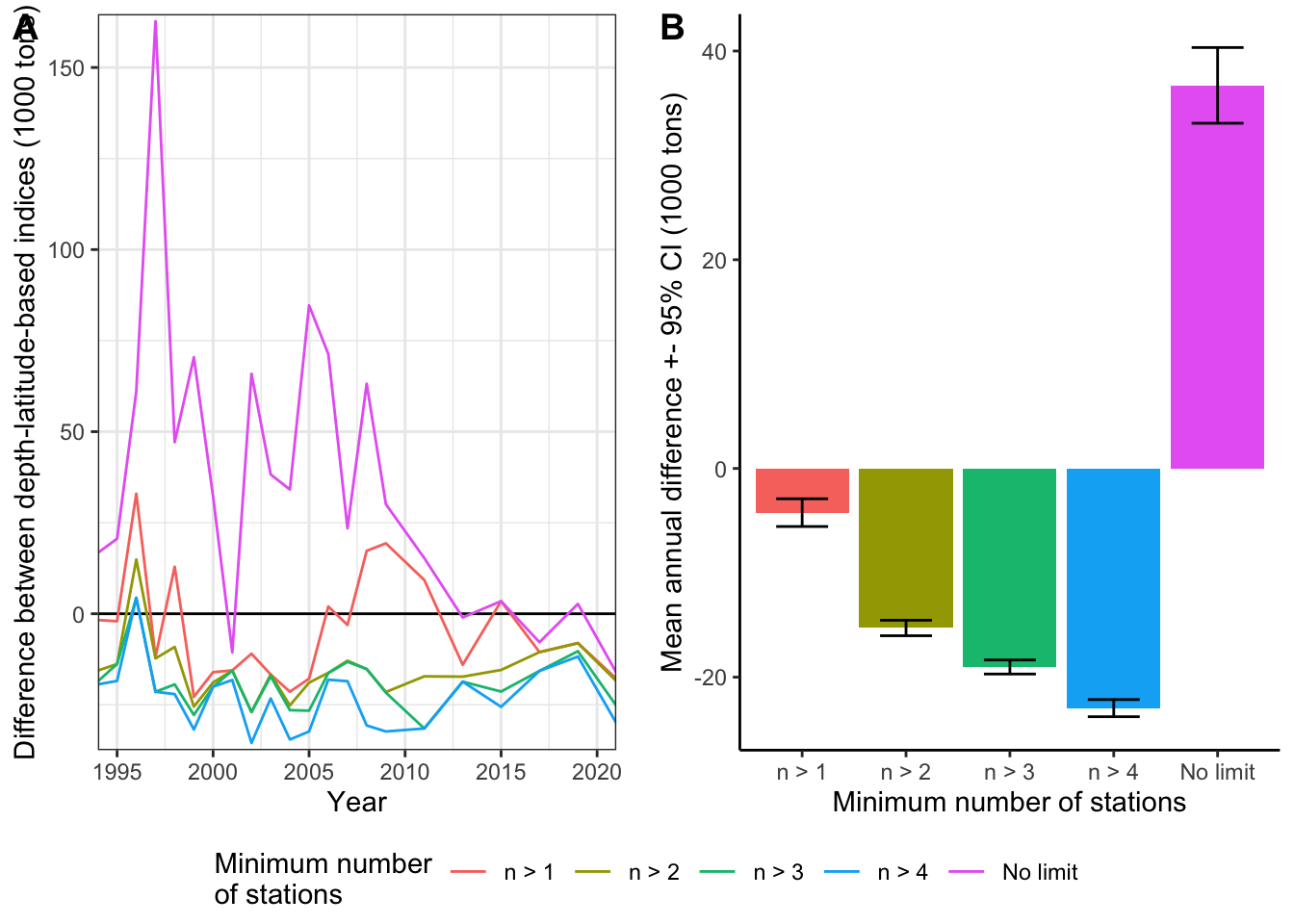
Figure 11: The influence of outliers on the difference between the depth-latitude-based indices calculated using the official (old) and reconstructed strata areas. Threshold for minimum number of stations per strata is indicated using color. A) Differences among years. B) Annual mean differences. Error bars indicate 95% confidence intervals assuming normal distribution.
Biadf
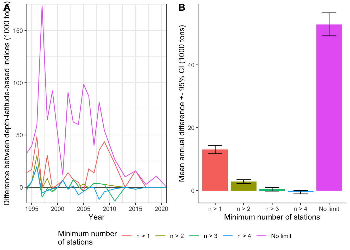
Figure 12: The influence of outliers on the difference between the depth-latitude- and position-based indices calculated using the reconstructed strata areas. Threshold for minimum number of stations per strata is indicated using color. A) Differences among years. B) Annual mean differences. Error bars indicate 95% confidence intervals assuming normal distribution.
Consequently, this alternative was used in depth-latitude and position-based station assignment comparisons.
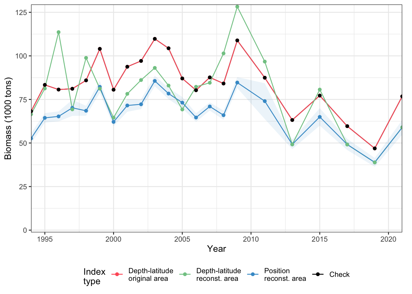
Figure 13: Blap
Number of stations per strata
Impact of geo- and depth strata on the index figure
Correlation between geo- and depth strata figure