Gallery of strata system examples

Introduction

This document contains examples of strata systems generated for various species needed by the author. The decisions behind the strata systems are not justified here and this document should be seen as a show piece of how the package can be used and a gallery for people working with stock assessment at IMR.

Setup

We use General Bathymetric Chart of the Oceans 15-arcsecond 2021 grid as bottom depth information to model the vertical distribution of the species. Since the file is 7.5 Gb, it is best to download the file to a central location on your computer and refer to that position instead of including the file in every project:

link <- "~/Downloads/gebco_2022/GEBCO_2022.nc" # Link to bathymetry data

Packages required to run the examples:

library(RstoxStrata)
library(dplyr)
library(ggOceanMaps)

Examples

Northeast Atlantic Greenland halibut

The strata system has been made for the new NEA Greenland halibut assessment model to be reviewed in a benchmark in February 2023. The system combines all previous strata systems that were developed separately for each survey time series. Geostrata has been adjusted to survey coverage, approximate country borders and distribution of the species along the Norwegian Coast and in the Barents Sea.

geostrata.df <- read.table(
  text =
  "name lon.min lon.max lat.min lat.max
1     A     0.0    10.0    62.0    64.0
2     B     0.0    14.0    64.0    67.5
3     C     8.0    18.0    67.5    70.0
4     D    12.0    18.0    70.0    74.5
5     E     4.0    16.8    74.5    77.0
6     F     4.0    16.8    77.0    79.8
7     G     0.0    25.0    79.8    83.0
8     H    18.0    36.0    70.0    72.3
9     I    18.0    36.0    72.3    74.5
10    J    16.8    36.0    74.5    77.0
11    K    25.0    36.0    77.0    83.0
12    L    36.0    54.0    69.0    74.5
13    M    36.0    54.0    74.5    77.0
14    N    36.0    50.0    77.0    83.0
15    O    50.0    80.0    77.0    83.0")

plotGeostrata(geostrata.df)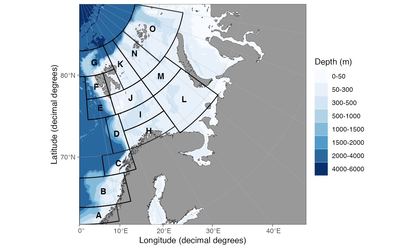

Depth intervals from existing survey indices. Boundary vector encompassing the area of interest to reduce the processing time.

depths.vec <- c(100, 300, 400, 500, 700, 1000, 1500) # Depth strata
boundary.vec <- c(0, 90, 62, 83.2) # Boundaries of the system

Fragment area (in \(km^2\)) is defined by trial and error.

strata <- strataPolygon(
  bathy = link,
  depths = depths.vec,
  boundary = boundary.vec,
  geostrata = geostrata.df,
  fragment.area = 1e4
)

## Plot 

plot(strata)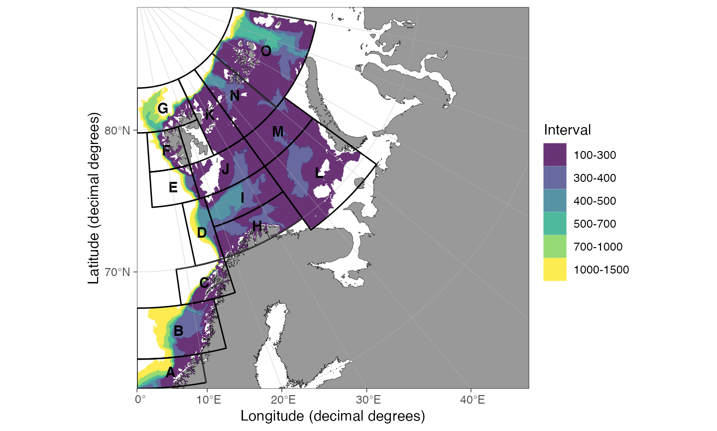

Greater argentine in the North Sea

geostrata.df <- data.frame(lon.min = c(3.2, 3.2, 7), 
                           lon.max = c(5.4, 7, 13), 
                           lat.min = c(59, 57, 57), 
                           lat.max = c(60, 59, 59.2)
)

depths.vec <- c(100, 200, 300, 500, 1000)

boundary.vec <- c(3, 13, 57, 61)

## Strata polygons vs. stations ####

pols <- strataPolygon(
  bathy = link, 
  depths = depths.vec, 
  boundary = boundary.vec,
  geostrata = geostrata.df,
  fragment.area = 100
)

## Plot 

plot(pols)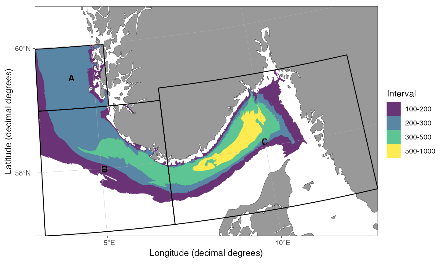

There are no stations in the shallowest strata of A and the function fails to remove a small fjord fragments:

pols$strata <- pols$strata %>% filter(!(geostrata.name == "A" & to == -100))
pols$strata <- smoothr::drop_crumbs(
  pols$strata, 
  units::set_units(50, "km^2", mode = "standard")
)

plot(pols, facetted = TRUE)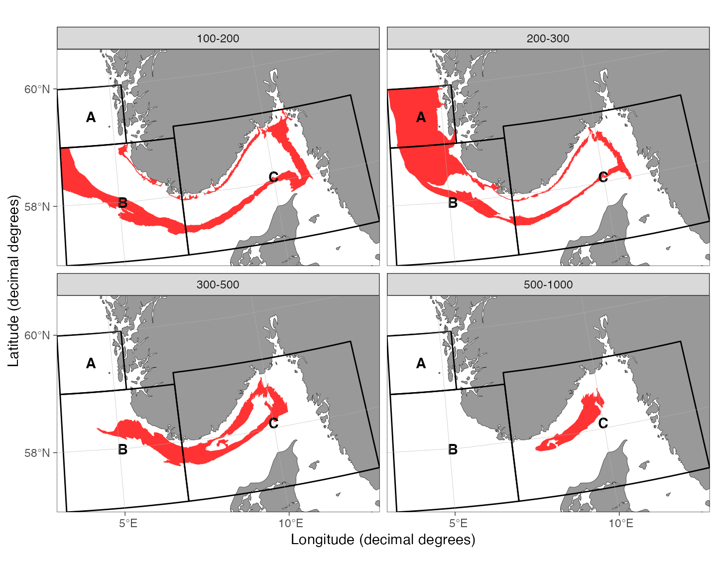

Greenland halibut continental slope, Norway (EggaNord)

This strata system attempts to mimic the strata system for EggaN survey index used in AFWG 2021 assessment as closely as possible. The calculus for the strata area used in stock assessment have been lost and they are not reproducible.

geostrata.df <- data.frame(
  lon.min = c(3, 10, 10, 8),
  lon.max = c(16, 17.3, 17.3, 17.3),
  lat.min = c(76, 73.5, 70.5, 68),
  lat.max = c(80, 76, 73.5, 70.5)
)

depths.vec <- c(400, 500, 700, 1000, 1500)

boundary.vec <- c(0, 17.3, 68, 80)

pols <- strataPolygon(
  bathy = link, 
  depths = depths.vec, 
  boundary = boundary.vec,
  geostrata = geostrata.df,
  fragment.area = 400
)

plot(pols, facetted = TRUE)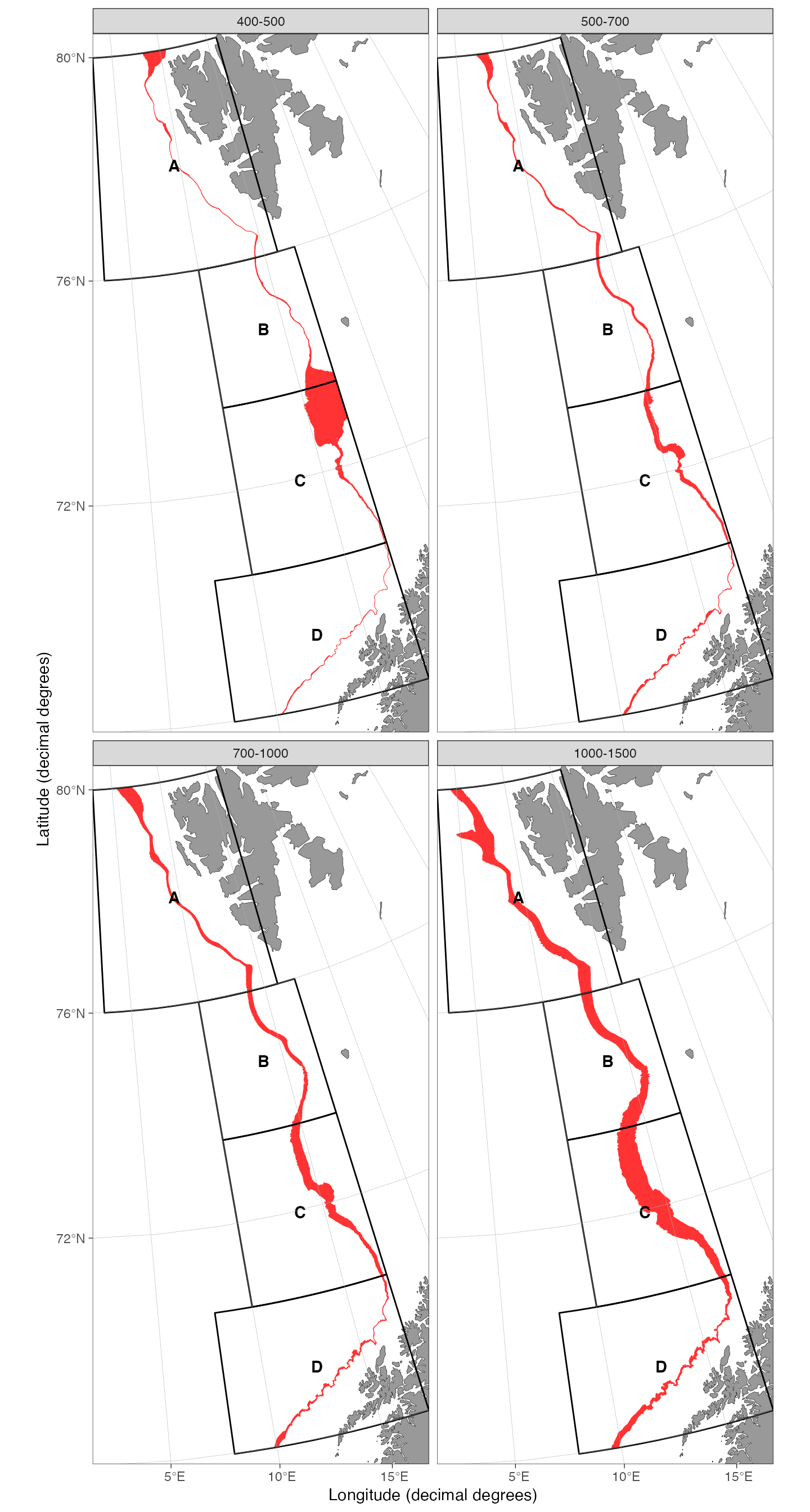

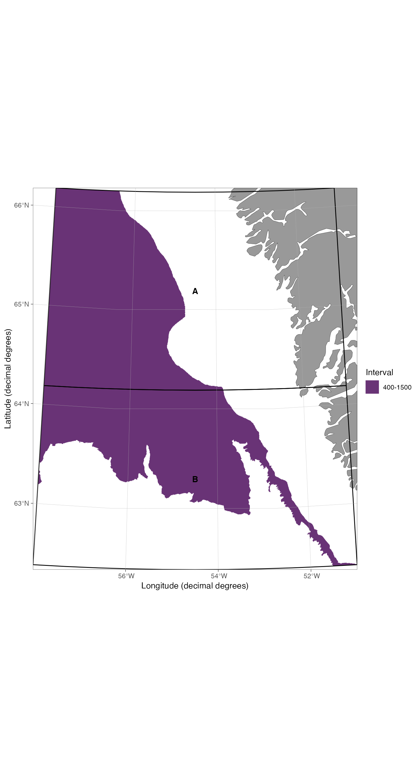
Greenland halibut in West Greenland

geostrata.df <- data.frame(
  lon.min = c(-58, -58),
  lon.max = c(-51, -51),
  lat.min = c(64.2, 62.4),
  lat.max = c(66.2, 64.2)
)

depths.vec <- c(400, 1500)

boundary.vec <- c(-58, -51, 62, 67)

pols <- strataPolygon(
  bathy = link, 
  depths = depths.vec, 
  boundary = boundary.vec,
  geostrata = geostrata.df,
  fragment.area = 1000
)

plot(pols, rotate = TRUE)

Mikko Vihtakari (Institute of Marine Research)

10 November, 2022