Map predicted densities from an sdmTMB model

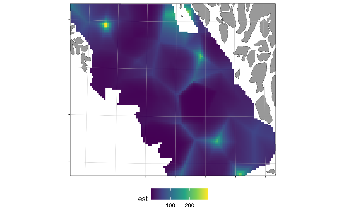
Maps predicted response values from stats::predict() output on a ggOceanMaps::basemap(), either averaged over time (type = "mean") or faceted by time (type = "annual").

Usage

plot_prediction_map(
  pred,
  crs,
  column = "est",
  type = c("mean", "annual"),
  time_col = "year",
  transform = "identity",
  fill_limits = NULL,
  xy_cols = c("X", "Y"),
  coord_multiplier = 1000,
  base_size = 11
)

Arguments

pred

A prediction data frame from predict(fit, newdata = ...), containing coordinate columns and the response column. If the response column is on the link scale (the default predict() output, e.g. log density for a log-link family), it can be negative; combine with a suitable fill_limits if you want to floor the colour scale, or use predict(fit, newdata = ..., type = "response") for density-scale values.

crs

Coordinate reference system (projected, in metres).

column

Character. Name of the response column. Default "est".

type

Character. "mean" (default) or "annual".

time_col

Character. Name of the time column (for type = "annual"). Default "year".

transform

Character. Fill-scale transformation, passed to transform in ggplot2::continuous_scale() (the successor to the now-deprecated trans argument). Default "identity".

fill_limits

Numeric vector of length two (either element may be NA), passed to limits in ggplot2::continuous_scale(). Values outside the limits are mapped to NA by ggplot2 and rendered as blank/grey cells. Default NULL: the scale's range is taken from the data, so no cells are dropped. Set e.g. c(0, NA) to floor a response-scale plot at zero.

xy_cols

Character vector of the coordinate columns. Default c("X", "Y").

coord_multiplier

Numeric factor to convert coordinates to CRS units. Default 1000.

base_size

Numeric. Base font size. Default 11.

Value

A ggplot object.

See also

ggOceanMaps::basemap(), ggplot2::continuous_scale()

Author

Mikko Vihtakari

Examples

# \donttest{
mesh <- sdmTMB::make_mesh(sdmTMB::pcod, c("X", "Y"), cutoff = 20)
m <- sdmTMB::sdmTMB(
  density ~ 0 + as.factor(year), data = sdmTMB::pcod, time = "year",
  mesh = mesh, family = sdmTMB::tweedie()
)
nd <- sdmTMB::replicate_df(sdmTMB::qcs_grid, "year", unique(sdmTMB::pcod$year))
pred <- predict(m, newdata = nd, type = "response")
plot_prediction_map(pred, crs = 32609)

# }